Biodiversity Patterns - RARITY

(see pg. 142-145 in text)

We should recognize that the species approach, while it is inadequate on the larger scale of conservation goals, can be important in identifying vulnerable species. To this end, Deborah Rabinowitz (1981, 1986) described a general pattern of species abundances, in which there were 7 different ways that species could be rare as described by scientists studying them. Rarity is in some of those cases, in the eye of the local beholder. Here is a table, essentially duplicated from the text, indicating how species can appear to be rare, be adapted to widely distributed low population densities, etc.

 
 Geographic range
 Large  Small
 
      Somewhere   Common       Locally         Locally         Locally
 large                    abundant over   abundant in     abundant in a
 a large range   several         specific
Population                     in a specific   habitats, but   habitat, but
Size                           habitat type    restricted      restricted
                                               geographically  geographically
 
      Everywhere Constantly    Constantly      Constantly      Constantly
 small     sparse over   sparse in a     sparse and      sparse and
 a large       specific        geographically  geographically
 range and in  habitat, but    restricted in   restricted in
 several       over a large    several         a specific
 habitats      range           habitats        habitat
 _____         __________      _____           __________
 Broad Restricted  Broad Restricted
 
 Habitat Specificity
 

Rabinowitz and her colleagues checked the patterns of distribution and local abundance for the species sufficiently well described in the flora of the British Isles. This flora has been studied and collected for literally hundreds of years. It has also been carefully mapped. From maps of individual species, it was possible to determine which species had large geographic ranges and which small (N.B. within the British Isles). Global species maps might alter the characterization of some species). From descriptions of habitats where species had been collected, fellow scientists were asked to decide whether the species were habitat specialists or generalists, as well as whether species were at least somewhere locally abundant. The kinds of descriptions are demonstrated below.

Descriptions:

Marshes, fens, heaths, woodlands, and waste ground. A common weed of arable land. – this is a description clearly for a habitat generalist, at least some places locally abundant.

Restricted to soil-filled crevices in scree slopes. – this is clearly the description of a habitat specialist.

Scarce where present. Occurs as widely scattered individuals.

– this is equally clearly the description of a species that is everywhere scarce.

  The table of relative occurrence frequencies for different kinds of rarity is shown below. There are two numbers in each cell. The first includes all species for which sufficient information was available, and for which there was general consensus among observers. The numbers in parentheses reflect more conservative criteria for inclusion, where 3 dissenting opinions or a consensus that the descriptions were ambiguous for any trait resulted in exclusion of the species. Statistical tests suggest that the two patterns ('liberal' and 'conservative' rules for inclusion) do not differ significantly. Also interesting is a test that indicates the three 'traits' are statistically independent. Think about that one. There seem to be logical links among these traits, so that they should not be independent. Common sense ecology would likely suggest that habitat generalists ought to be widespread in distribution, but there are habitat generalists with narrow (small) range. Logic that is not quite so strong might also suggest that widespread species should be at least somewhere locally abundant, but there are exceptions to this as well.

 
                            Geographic range
 Large Small
Somewhere                                                       
 large      58 (21)        71 (23)           6 (0)          14 (4)
 
Population
Size
 
Everywhere    2 (0)          6 (0)            0 (0)           3 (1)
 small _____      __________           _____        __________
 Broad     Restricted            Broad        Restricted
                           Habitat Specificity
 

Thus, Rabinowitz argued that species rarity could occur in three different ways: 

1) restricted geographic distribution;

2) narrow habitat distribution;

3) low local population abundance.

Of the British flora analyzed, 39% had no component of rarity (i.e. they were not rare in any way), while among the 61% that were rare in one or more ways:

59% had narrow habitat specificity;

15% had small geographic range;

7% had low population size.

How one divides abundances and ranges into abundant/rare, large and small affects one's results.  Pitman et al. (1999) analyzed trees in Peruvian Amazon forest, and set 1 ind./ha as the abundance dividing line, 1 vs. 2 or more forest type occurrences for habitat breadth, and a political boundary (Madre de Dios) for geographic distribution.

This analysis showed that none of the trees were geographically confined (no small geographic ranges), and only 13% were locally rare. The rarest trees occurred at 1 stem per 36 Ha; over this forest this 'rare' species would encompass 200,000 stems!  One important consequence of this result is, however, that conservation of truly rare species will require preservation of a lot of land (Rickelfs 2000).  Pitman et al.'s results also differ markedly from the British forests surveyed by Rabinowitz.  Much of this difference may relate to the spatial scale used; consideration of spatial scale is obligatory when assessing rarity. The lack of apparent habitat specialization by these tropical trees runs in contrast to prevailing views. They also stand in contrast to Rapaport's Rules that high tropical diversity is associated with habitat specialists and small geographic ranges.

  Why is the separation of forms of rarity important to conservation biology? Think about how the limited resources available for conservation should be spent. Whole countries identified as centers of diversity cannot be wholly conserved. Population, development, and politics make any thoughts of that level of protection ridiculous. Within such countries, what should be protected? Clearly, the best approach is to preserve habitats and ecosystems. But which ones? If information of this sort is available (or can be developed) for species of various sorts (not just plants), then the form of rarity can be very useful. A species that is rare due to limited geographic distribution, but has fairly generalized habitat requirements and is locally abundant seems like a good candidate for introduction into areas outside its current distribution limits. A species with a wide distribution and high local abundance, but narrow habitat requirements, probably cannot be successfully moved; it has likely already sampled areas throughout its range. The likely solution is protection of at least some of the local populations already established. Species that are locally sparse, but widely distributed and generalized in habitat requirements probably need no protection. In sum, species restricted to narrow niche characteristics in two or more of the three traits are those most likely to need some help. They can identify species, habitats, and communities on which to spend our efforts.

  There may exist biological reasons for species rarity. Kunin and Gaston (1993), in a review of rare and common species, found that rare species (i.e. locally rare and geographically restricted) differ from more common species.  Rare species have lower levels of self-incompatability, a greater tendency to asexual reproduction, lower overall reproductive effort and poorer dispersal abilities. In a sense, they tended to make the best of a bad situation.

Groups such as the World Conservation Union (IUCN) use indicators to determine which species are rare and at risk of extinction. Programs can then be developed for these species to alleviate their population persistence problem. Typical indicators used for this purpose include:

1) rarity;

2) rate of decline (high rates being bad);

3) degree of population fragmentation.

However, Hartley and Kunin (2003) have demonstrated that each of these 3 indicators is sensitive to the scale at which they are measured. Rarity can be measured using 3 metrics:

1) Extent of occurrence – essentially the total range area (this tells us nothing about the distribution of individuals within that range nor their abundance);

2) Area of Occupancy – typically measured by summing occurrence of individuals in individual ‘cells’ of a grid encompassing the entire range (again, telling us nothing about abundance at each);

3) Population Counts – measured by population census (highly specific population number for a specific location in the Area of Occupancy:

Area of Occupancy (AOO)

___________________________________________________________

Population Count (PC) Extent of Occurrence (EOO)

(individuals) (range size)

ß------------------------------------------------------------------------à

fine scale coarse scale

In the IUCN model, species are considered critically endangered if the extent of occurrence is <10km², endangered if they occupy <500km², and vulnerable if they occupy <20,000km² . A problem arises with the AOO criterion however, since species mapped at high spatial resolution will appear rarer than species mapped at coarser spatial resolution. This means we are more likely to give lower extinction risk values to species for which we have the least information (Hartley and Kunin 2003). In Britain, AOO is measured on a 100 km² grid, meaning that species occurrences can only be mapped at no less than this level of resolution (i.e. they cannot be called critically endangered since no measures at the high spatial resolution scale are available).

Using measures of rate of decline is also fraught with problems. As the term implies, rate of decline will be measured by assessing population size over at least 2 points in time. Four possible measures are possible using only range size and population number (declines in range but not population number, declines in population number but not range, both, neither). Field evidence suggests that calculations based on decline at the coarse scale (AOO) would yield lower decline rates than those calculated at a fine scale (PC).

Third, the IUCN method also considers population structure with respect to dispersal potential (i.e. fragmentation extent). However, severe fragmentation (many small, isolated populations) and lack of fragmentation (a single or few subpopulations) can be considered as indicative of increase risk of extinction. So, the relationship between fragmentation and risk is not clear. Thus all three criteria currently used by IUCN to designate species are endangered or not as sensitive to spatial scale problems.

Hartley and Kunin (2003) note that 3 options exist for dealing with spatial scale issues:

1) Use a standard spatial scale to measure AOO – e.g. the 100 km² as in Britain, even though it has problems.

2) Measure each of the 3 metrics across as many spatial scales as possible (basically Rabinowitz’s approach). It overcomes the issue of arbitrary scale size selection, which may or may not reveal true rarity. But it requires and produces a great deal of information.

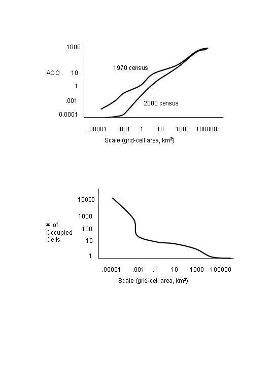
3) Combine information from multiple scales in a simple, unified, quantitative manner by plotting AOO vs. scale size.

Figure 4 – Hartley and Kunin (2003)

If we plot the AOO values for more than 1 time period on the graph, we can determine whether the curves have changed and whether the species is becoming more rare, and, if so, at what spatial scale. If we use the multiscale approach, as suggested by Hartley and Kunin (2003), we will be able to calculate the value of each rarity metric and at any scale, and therefore determine precisely how a species’ abundance and occurrence are changing over time.

References

Harte, J. and E. Hoffman. 1989. Possible effects of acidic deposition on a Rocky Mountain population of the tiger salamander Ambystoma tigrinum. Conservation Biology 3:149-158. 

Hartley, S. and W. Kunin. 2003. Scale dependency of rarity, extinction risk, and conservation priority. Conservation Biology 17: 1559-1570.

Kunin, W.E. and K.J. Gaston. 1993. The biology of rarity: patterns, causes and consequences. TREE 8:298-301.

Pitman, N.C.A. et al. 1999. Tree species distributions in an upper Amazonian forest. Ecology 80:2651-2661.

Rabinowitz, D. 1981. Seven forms of rarity. pp. 205-217 in The Biological aspects of rare plant conservation. Ed. by H. Synge. Wiley.

Rabinowitz, D., S. Cairns and T. Dillon. 1986. Seven forms of rarity and their frequency in the flora of the British Isles. In M.E. Soule; (ed.) Conservation Biology:  The Science of Scarcity and Diversity. pp. 182-204. Sinauer.

Ricklefs, R.E. 2000. Rarity and diversity in Amazonian forest trees. TREE 15:83-84.