The Basic Model of Island Biogeography
The model is one of a dynamic equilibrium
between immigration of new species onto islands and the extinction of species
previously established. There are 2 things to note immediately: 1) this is a
dynamic equilibrium, not a static one. Species continue to immigrate over an
indefinite period, not all are successful in becoming established on the
island. Some that have been resident on the island go extinct. The model
predicts only the equilibrium number of species, will remain 'fixed'. The
species list for the island changes; those changes are called turnover. 2) The
model only explicitly applies to the non-interactive phase of island history.
Initially, at least, we will consider only events and dynamics over an
ecological time scale, and one which assumes ecological interactions on the
island occur as a result of random filling of niches, without adaptations to
the presence of interacting species developing there. Evolution is clearly
excluded.
The
variables used in the basic model are Is,
the immigration rate, which is clearly indicated by the subscript to be species
specific, i.e. to be dependent on the number of species already present on the
island. Here we're not counting noses, but rather the rate at which new species
(those not already present on the island) immigrate. Phrased explicitly, it is
the number of species immigrating per unit time onto an island already occupied
by S species. Also Es, the extinction rate, measured in species lost
per unit time from an island occupied by S species. Finally, we need to know
the size of the pool of species in the source area available to colonize the
island.
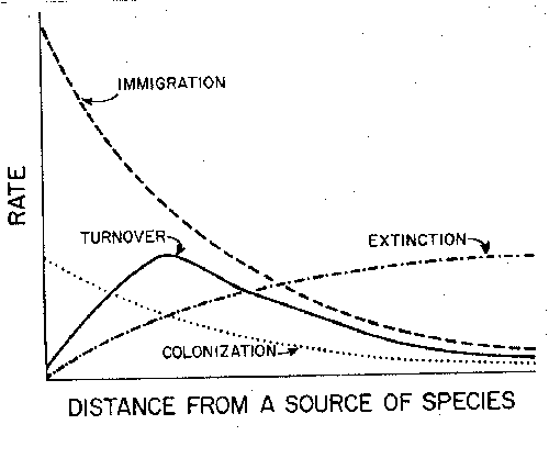
The immigration rate Is must certainly
decrease monotonically (on average) as the number of species on the island
increases, since as S increases there are fewer and fewer species remaining to
immigrate from the pool P of potential immigrants at the source. If all species
were equally likely to immigrate successfully (i.e. had equal dispersal
capabilities), but actual immigrations were chance events, then the
relationship between Is and S would be
linear, the probability of a new species immigrating would be directly
proportional to the number of species left to arrive. There are, however,
considerable differences in the dispersal abilities of species in source areas.
Those with the highest dispersal capacities are likely to colonize an island
rapidly (have a higher immigration rate), and later, on average, those with
lower dispersal capacities will follow. They will not only immigrate later, but
the rate at which they immigrate will be lower because they have lower
dispersal capacities. The rate at which species accumulate on islands is,
therefore, initially rapid and then slower. Also, among those species with
lower dispersal capacities the successful immigration of any one species should
have less effect on the immigration rates of species remaining in the source
pool (we have not removed a likely immigrant from the pool) than would the
earlier immigration of a highly dispersible species. Therefore, this part of
the curve should be 'flatter'; the rate of immigration should be little affected
by the arrival of one of these poor dispersers. The result is an observed
immigration rate curve which is concave. The actual (or theoretical) curve for
any island is dependent on its isolation. For any source pool, the observed
rate, while similar in shape, will be lower for more distant islands than for
closer ones. Immigration rates are graphed from the left hand edge of figure 1,
declining from the y axis with an increasing number of species already present.
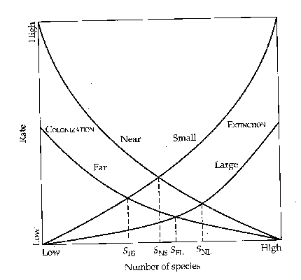
Figure
1 - The basic graphical model of equilibrium in the MacArthur-Wilson model.
Figure from Brown and Gibson -Biogeography.
The extinction rate Es should be, from
parallel reasoning, a monotonically increasing function of S. If area, for
example, acts only through its effects on population sizes, and extinctions are
the chance result of small population sizes and demographic stochasticity,
then as the number of species increases, the number of species with small
populations and subject to chance extinctions increases in proportion, i.e. the
relationship would be linear. However, if we consider a more realistic
biological scenario, then as the number of species increases, depressant
interactions within and between species (competition, predation, parasitism) are more likely to occur, and extinctions are
more likely as a result. Remember that these are not species that have evolved
adaptations to interactions. Effects are direct and unmoderated.
Since any extinctions resulting from interaction are in addition to those
resulting from demographic stochasticity, the more
realistic shape for the extinction curve is concave upwards. The extinction
rate begins at 0 when there are no species on the island, then
increases as species accumulate. At least for purposes of simplicity in looking
at the basic implications of the model, the extinction curve can be thought of
as a mirror image of the immigration curve.
We
now have all the information to produce the basic graphical model. That model
predicts that there is some value of S, which is called Ŝ, for which
immigration rate and extinction rate are in balance; there is a dynamic
equilibrium. At that diversity on the island species are immigrating at a rate
equal to disappearances due to extinction. The result is constant change in the
species list on the island; that change in names occurs at a rate called x, the
turnover rate. The length of the species list, however, should remain constant.
This is a stable equilibrium since, should something happen, and the number of
species on the island be perturbed, the imbalance between immigration and
extinction rates at the new S would tend to return island diversity toward its equilibrium
value. Below Ŝ additional species accumulate; immigration rate is larger
than extinction rate. Above Ŝ the reverse is true, extinctions exceed
immigrations and the number of species declines to Ŝ.
Tests of the Model
To
test the model, an important piece of evidence is a carefully designed
manipulative experiment studying the fauna which colonize 'islands'. One of
Wilson's students, Dan Simberloff, tested the model using islands which consist
of mangrove mangles in the Florida Keys. Simberloff's
Ph.D. thesis had consisted of measurements of the re-colonization of these
islands following 'defaunation' (he had encased
individual mangles in giant plastic bags, sprayed them with short acting, low
persistence insecticides, then followed the rates, numbers, and species which
immigrated onto them after exposure). Re-equilibration, i.e. reaching a stable
number of species, had occurred within 3 years of fumigation in his earlier
experiments. In a second series of studies (Simberloff 1976), the manipulations
were equally inventive. After the
islands had been censused, and an equilibrium number
of species determined for each island (a 'control' diversity), crews moved in
with chain saws, handsaws and hatchets, and each island was split into 2 or
more smaller parts, with water gaps of 1m between. To the insects, apparently
this 1m gap was sufficient to make crossing from one sub-island to another a jump dispersal. The smaller, sub-islands were then censused repeatedly over a time interval sufficient to
permit re-equilibration to find out how species numbers changed with island
area. Remember, the area censused had been part of a
previous island, and should contain all habitats (plant parts, vertical
structures) in the same proportions as before (i.e. the same habitat
heterogeneity, however measured). Alterations were only quantitative, in the
form of area reduction, no unique feature was removed.
The
results were clear-cut. Each island reduced in size re-equilibrated at a lower
insect diversity. Considering all the experimental islands in developing a
model for the pattern in reduction, the diversity change fit a log-log
relationship (i.e. a power function) between diversity and area. Thus, Simberloff's data fit the original species-area
relationship. Area was the key determinant. The process of re-equilibration,
however, involved extinction of species from islands supersaturated due to
their reduction in size. We have already encountered the underlying biological
cause of those extinctions: population sizes of 'marginal' species,
that is those whose populations were already small before reduction in
area, were decreased to the point where chance extinction due to demographic stochasticity became likely, and re-colonization unlikely.
Such extinctions are an important component of the equilibrium model of island
biogeography.
Figure
2 - Effect of island fragmentation on insect diversity in mangrove mangles.
Simberloff (1976).
There
are few islands that have been studied over long enough periods to test the
hypothesis of equilibrium with turnover, i.e. the occurrence of a stable but
dynamic equilibrium. Among those few are the California Channel Islands. The
interpretation of these data is a source of continuing controversy. That's
important, because the crux of the equilibrium theory is proof (or
documentation) of insular turnover at equilibrium. A paper (Gilbert 1980) found
25 attempts to document turnover at equilibrium, and found few (basically just
mangrove island studies by Simberloff) acceptable without question. In Simberloff's original defaunation
studies, for example, one island supported 7 species of Hymenoptera prior to
fumigation and 8 after equilibrium had been re-established about one year
later. However, only two of these species were present both before and after
fumigation. This sort of experimental study is designed to allow for rapid
re-equilibration.
The
Channel Island studies represent an interesting attempt to deal with the
problems of scale (here time) when dealing with most real ecosystems.
Recognizing that there may be difficulties (the initial, historical survey of
species presences on the island used breeding records collected over many
years, rather than a single survey at one time), Diamond's studies of turnover
on the Channel islands are still regularly cited (Diamond 1969).
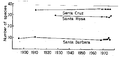
Initial
data reported collections and observations indicating the fauna of individual
islands in 1917. Diamond compared those species lists with a survey he did in
1968. Over the 51 years between censuses the numbers of species on islands
remained almost perfectly constant, but turnover was as high as 62%, i.e. as
much as 62% of the original list had been replaced by new species. The islands
had the following characteristics:
Island 1917 1968 Extinctions Immigrations %turnover
Los Coronados 11 11 4 4 36
San Nicholas 11 11 6 6 50
San Clemente 28 24 9 5 25
Santa Catalina 30 34 6 10 24
Santa Barbara 10 6
7 3 62
San Miguel 11
15 4 8 46
Santa Cruz 36
37 6 7 17
Anacapa 15 14 5 4 31
These data seem initially to
fit the equilibrium theory quite well. Numbers remain almost constant while
turnover occurs in a significant number of species. However, the theory also
suggests, as you will soon see, that turnover should be related to island area
(through effects of area on extinction rates) and/or isolation (through effects
on immigration rates. Neither was the case; instead turnover was approximately
inversely proportional to the number of species present. That is not forecast
by the model.
Figure
3 - The number of species in censuses of 3 of the California Channel
Islands.
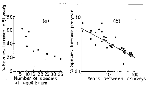
Figure
4 - % turnover in species numbers on California Channel Islands. (a) for nine of the islands. (b) for Anacapa as a function of time between pairs of surveys.
Why
should turnover be related to island area or isolation? Consider first 2
islands at equal distance from the source, but differing in area. Long distance
(jump) dispersal is generally assumed to be a chance event, not directed or
goal oriented. In that case, dispersal probabilities and immigration rates onto
the 2 islands should be the same. Area, however, does affect the extinction
rate of colonists. The larger island should have 1) higher habitat
heterogeneity, 2) decreased intensity of interactions due to reduced niche
overlaps resulting from habitat heterogeneity and 3) larger population sizes
making chance extinctions less likely.
These
factors should be operative, at least in a relative way, independent of the
number of species present. Therefore, the extinction curves should have similar
shape, but have lower values for the larger island. Putting this comparison on
a graph, but using a linearized version of immigration
and extinction curves, we find a larger equilibrium number of species on the
larger island, but also a lower turnover rate on that island.
To
assess the effects of isolation consider 2 islands of equal size, but located at
differing distances from the source. With identical sizes we assume that
habitat heterogeneity, population sizes and interactions on the islands are
quantitatively identical, and thus they have the same extinction rate curves.
Immigration rates onto the more distant island should, however, be lower at any S since the probability of a successful
dispersal decreases (possibly exponentially) with distance. We can go further,
and suggest that the decrease should be most noticeable for species which tend
to be among the first colonists. Later immigrants with lower dispersal
capacities have only a slim chance anyways, and depend on rare, special
conditions like storms for successful immigration. For these species a change
in distance should mean less in shifting immigration rates. Once more we turn
these suggestions into a comparison on the graph. The more distant island has a
lower equilibrium number of species, but also a lower turnover rate at
equilibrium than an island closer to the source.
Figure
5 - Multiple immigration and extinction curves indicating effects of
differences in size and isolation on equilibria and
turnover rates. Brown and Gibson (1983).
These
comparisons can be combined in various interesting and complicated ways. Rather
than document the possibilities, it is probably more valuable to attempt to
list the assumptions and predictions of the basic MacArthur-Wilson model. Some
of the ideas in this list will not be fully examined until later in this
section.
Under What Conditions Does the Model Apply?
1) Islands are real isolates (rescue
effect, discussed below, not important)
2) Islands have comparable habitat
heterogeneity (complexity). There are no gross environmental changes over the
time period of colonization
3) Species counted on islands are
residents
4) There is a definable mainland species
pool
What Are the Characteristics of the Equilibrium?
1) It is dynamic
2) It is approached asymptotically
3) The process is inherently stochastic
4) The model and the equilibrium are
describing processes in ecological time
What Are the Characteristics of Turnover?
1) The process is not successional
2) Species replacements occur frequently
3) Immigration rates decrease with
increasing species numbers. Extinction rates increase with increasing species
numbers
What Influences the Equilibrium Number of Species?
1) Influenced by area through extinction
rates
2) Influenced by isolation through
immigration rates
3) Varies faster with area on distant
islands (see below)
4) Varies faster with isolation on small
islands (see below)
With this summary in mind, we return to problems.
With regard to Diamond's data, no combination of size and isolation leads to
the prediction that turnover rate is inversely (or in any other sense)
proportional to the number of species on an island.
Since
the data are repeatedly cited and classic, it's worth trying to understand why
this anomalous result was reported. There are a number of possible answers, and
arguments in the literature could be described by indicating that 'the fur has
definitely flown'. For one thing, the interval between the censuses was very
long. That may have had significant effect on the measured turnover. If the
time interval is long enough it becomes likely that some of the species which
had gone extinct at some time between the censuses also re-immigrated during that
interval (or the converse). In either case the measured turnover would
underestimate actual rates. To attempt to correct for that possibility, Diamond
and his collaborators went back to the Channel Islands annually during the
early 1970's, and also used thorough data gathered for Farnes
Island off Great Britain. The result of differences in the interval between
censuses is evident in Fig.8 (and reported in Diamond and May 1978). The result
for the Farne Islands is parallel. In either case the
apparent turnover decreases rapidly as the census interval increases. To show
you why, consider what happened to the meadow pipit on Farnes
between 1946 and 1974 (May and Diamond 1977). The pipit bred for 2 years, went
extinct in the 3rd, then went through 5 more cycles of
immigration and extinction over the remainder of the period. From annual census
records that indicates 11 turnover events in 29 years, where a census after 30
years would have recognized only a single extinction, as well as a constant
diversity of 6 species on the island. The same basic pattern applies to the
Channel Islands. Instead of turnover rates ranging from 17-62% (or .34-1.24%
per year), annual censuses indicate actual turnover rates of 1-10% per year,
and are about an order of magnitude larger than indicated by to 51 year
interval for most islands.
That's not the only corrective surgery which
has been suggested for the theory. It is also evident that monotonic rate
functions (particularly the immigration rate curve) may be overly simplistic.
That should be evident by drawing a parallel between accumulation of species on
an island and primary succession. When an island is newly formed (frequently
volcanic) it has no organic content in (and frequently no) mineral soil. The
first plants must be special sorts that have no requirement for nutrients from
the soil (or possibly no requirement for soil at all); instead they are soil
formers, leaving behind their nutrients extracted from the rock (as well as
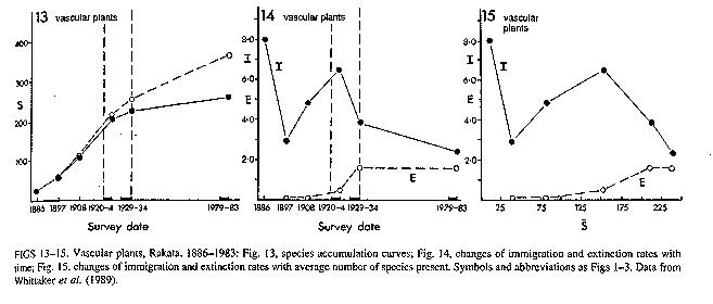
their bodies) to improve conditions for later arrivals. Krakatoa,
East of Java, was not only a B movie, but a real historical event in the
1880's. What kind of immigration curve described the relationship between
immigration rate and the number of species on Krakatoa
after its formation. Depending on our definition of
immigration (does it end with landing on the island, or require initial growth
to be counted) and extinction (does a species have to reproduce at least once
on an island before we consider its loss an extinction?)
either immigration rate or extinction rate curves could be modified. For
simplicity we'll include the modifications in the immigration rate curve. Now it isn't monotonic decreasing; instead it
may have an initial rising phase representing the additional immigration possible
with the formation of soil. That is the naive logic. Reality isn't quite so
simple. Over the first 50-60 years since eruption (1883) the 'curves' of the
number of species accumulated over time for various plant groups seem virtually
straight lines; there is no decrease in rate of immigration over this time.
Similar arguments could be advanced, producing a similar curve shape, with
respect to other trophic levels. Equilibrium diversity and turnover rates can
be affected by these modifications.
Figure
6 - Colonization rates for vascular plants on Krakatau
measured in terms of total number of species (labeled 13), immigration and
extinction rates (14), and as functions of the number of species present (15). From Thornton et al. (1993).
Since
Diamond's data from the Channel Island studies suggested an appropriate
relationship between turnover and area-isolation effects, but could not
quantify them, an appropriate experimental test became important. Jim Brown and
his wife Astrid attempted such a test (Brown and Brown 1977). They studied the colonization of thistle
plants by assorted insects and spiders by repeated census following defaunation. Almost everything fit the basic
MacArthur-Wilson model, but... The turnover rate should be inversely related to
island distance (isolation) according to the theory. If we look at just
distance effects on the same island (i.e. area), the nearer island should have
a higher turnover rate. That's not what the Browns found. Instead, whether
plant 'islands' were large or small the turnover rates were higher on more
distant islands.
Site 1 Site 2
# of
plants Mean # species turnover rate # of plants Mean # species turnover rate
large- 16 3.82 0.67 9 5.25 0.29
near
large- 7 3.78 0.78 9 4.44 0.42
far
small- 56 1.89 0.78 21 2.21 0.69
near
small- 3 1.33 1.00 11 0.80 0.91
far
Based upon a 5 day census interval (remember what
Diamond's data ended up showing about the importance of census interval),
turnover rates were consistently higher on the more isolated plants. This
reversal of the expected pattern is explained as resulting from the effect of
repeated immigration of species onto near islands. The original model was
psychologically, if not explicitly, concerned with a degree of isolation which
made such repeated immigrations unlikely. Under real conditions repeated
immigration may be likely, particularly on near islands. Addition of a new
immigrant member into a small population reduces the probability of extinction.
This repeated immigration is, therefore, termed the 'rescue effect'. It could,
as I've just suggested, be presented as affecting immigration or extinction, but
since the key effect is on extinction rates, making extinction less likely on
near islands, that's where the curves are usually adjusted for rescue. When the
rescue effect occurs, turnover rates will tend to be directly proportional to
distance. The effect may be evident in data sets as divergent as these studies
of plant 'islands' and Diamond's New Guinea satellite island avifaunas.
Figure
7 - How the rescue effect modifies curves of immigration, extinction, and
turnover as a function of distance.
From
predictions of rescue effect occurrence we can make some general, graphical
predictions of how distance effects immigration, extinction and turnover. Note
that we are here graphing these rates against distance, not against species
numbers. The immigration rate declines exponentially with distance, as we've
previously seen in a variety of data. The extinction rate was previously
considered as depending on island area, and unrelated to distance; it would
have been a straight horizontal line on this graph before we considered rescue.
Now we recognize that the rescue effect bends the extinction curve down at low
distances. When we combine these curves to estimate turnover as a function of
distance, it has an intermediate peak; turnover is highest at those distances
when both immigration and extinction rates are high. Very close to the source
extinction rates are low; at large distances immigration rates are low.
The
next correction to the simple model is one which questions the validity of the
species-area relationship. Are projections of area-dependent extinction valid
for the total range of island areas studied? Of course, I wouldn't be
suggesting the question unless something were amiss.
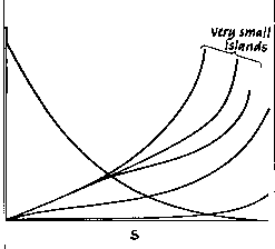
There is a problem on very small islands. MacArthur and Wilson recognized that
possibility in presenting the basic theory, and suggested such islands were
unstable, should have very high turnover rates, and probably not have area-dependent
extinction curves. Basically, they thought any area effects would be masked by
the instability of the islands. The figure in the original monograph showed a
split curve for extinction rates, i.e. an unpredictable area effect. The
original data used to construct that graph was drawn from studies of the
ecology of the Kapingamarengi atoll system in the
Carolina Islands in Micronesia (Niering 1963). These
small outcrops appeared to show a threshold in the species-area relationship at
about 3.5 acres in area. It was suggested that the instability was not habitat
destruction by physical forces, but instability in the presence of fresh water.
Below the threshold area the water table on the island is saline; fresh water
availability depends totally on frequent rains. Above the threshold area there
is a permanent 'lens' of fresh water, and extinction
of plant and animal species dependent on fresh water becomes much less likely.
Figure
8 - Predictions of extinction rate characteristics on very small islands.
From MacArthur and Wilson (1967)
That explanation seemed
fairly successful and biologically reasonable. However, Whitehead and Jones
(1969) re- examined the same data and came to somewhat different conclusions.
First, they found the data better fit by a curvilinear relationship between
species and island area, rather than a threshold. That, by itself, doesn't mean
too much. They also explored biological bases for the curvilinear relationship.
Their rationale were:
a) Part of
the problem was that the species list included a number of species introduced
by man. Almost all these species were found solely on larger atolls; a number
have been recent introductions. These species (particularly recent
introductions) are not part of a normal biological equilibrium, and removing
them from the species-area curve seems to lower the slope of the curve at
larger areas without affecting the slope among smaller atolls (fewer visits by
man means that there have been fewer introductions on smaller atolls). The way
removals from species lists were handled left those species apparently
introduced by Melanesian natives early enough to have had a reasonable
opportunity to have become part of a biological equilibrium or to have gone
extinct.
Figure
9 - An alternative view of characteristics of species contributing to
diversity on Kapingamarangi atoll. From Whitehead and
Jones (1969)
b) In
addition, there is more than one kind of species introduced to the islands by
natural dispersal. The different types also show different rates of numerical
increase with area. One kind is what are called strand
type species. Strand species are those which inhabit the relatively uniform
shoreline habitat. Most are salt tolerant both in dispersing and adult phases.
As adults they live in a habitat which is subject to frequent, if not
continuous, salt spray. As dispersers many, if not most, are passively carried
on ocean currents. These adaptations suggest that strand species do not require
a lens of fresh water, and would therefore have no area threshold for
occurrence. They also suggest that such species should be widespread and have a
relatively high immigration rate. Thus, including the presence of a rescue
effect, these species should have low extinction rates as well. In sum they
should show little area effect and low endemism. The data from Kapingamarangi indicates that even the smallest atolls,
only a few meters in diameter, have 5-7 species of the strand type, while the
largest islands, with areas measured in the tens of square miles, have only
12-14 such species. In essence, strand species have a species- area curve which
approaches a straight, horizontal line.
c) The
so-called non-strand species cannot tolerate salt water and persist only where
a lens of fresh water persists in the soil. Once the strand and introduced
species are cropped from the species lists, the remainder
(non-strand) display a species-area curve which fits quite well to the
predictions of the MacArthur-Wilson model. Thus the basic theory is compromised
by its inability to deal effectively (at least as a unified, simple model) with
ecologically heterogeneous species groups.
The basic theory arose from intensive study of avifauna and ponerine ants on widely spaced oceanic islands. Rooted in
studies of homogeneous taxa of limited underlying ecological variety
(particularly the ants, but in terms of dispersal and foraging methods,
probably birds as well), the theory fits such groups well. When extended to a
broader taxa and 'islands' the accuracy of predictions and the utility of the
basic model are called into question.
There is one last criticism to aim at the
basic theory before moving on to its quantification. Let's say you are studying
a group of islands which should equilibrate fairly rapidly, both because of
their distance from the source pool(s), their size, and the taxa under
investigation. Over time you find the number of species on the islands to vary,
even after it would seem that equilibrium should have been reached. What can
you conclude?
1) That Sob
is slowly approaching Seq, but that
equilibrium has not been reached due to disturbance, possibly at an intensity
subtle enough that the observer fails to note the disturbances - or -
2) That
equilibrium has, in fact, been reached, but that the equilibrium itself varies
due to shifting ecological conditions (e.g. climate) either on the island,
affecting extinction, or at the source, affecting immigration. As a corollary
of this view, even the observation of a constant number of species does not
ensure equilibrium, since we have no independent estimate of S. The simple
theory is simply not that quantitatively predictive as presently constituted.
That, in a nutshell, is the key problem of this theory. It is extraordinarily
difficult to design an experiment with appropriate controls on S, etc. to
falsify the basic model. Yet the model remains very important to a broadening
range of fields, subject to intensive efforts at corrective surgery, because it
does have a lot of qualitative predictive ability.
Modeling Effects of Disturbance on the Equilibrium
Theory
It is apparent that disturbance can have
important consequences for observed equilibria or the
lack thereof. What is difficult is the fact that disturbance has effects on the
survival and/or reproductive success of individuals. A disturbance, unless
extraordinarily massive, does not affect every member of a population. Modeling
on an individual basis has been difficult or impossible until recently. An
Italian group (Villa et al. 1992) attempted to evaluate the effect of regular
disturbance at differing intensities on the equilibrium. The following were
their conditions:
1) Island
habitats were equally distant from the 'source', but differed in size, from 50
'cells' (each cell was a potential site for an individual) to 1100.
2) The were 64 species. Each had its own mean lifespan,
interval between reproduction, and a range of clutch sizes from minimum to
maximum, i.e. a life history. Each species also has a relative dispersal
capacity.
3) A
colonization species pool with relative abundances in the pool set.
4)
Colonization occurs by randomly allowing individuals to disperse according to a
negative exponential distribution (but distributions are affected by relative
dispersal distance). They are successful if they land on an empty cell. If so
their life histories determine whether the population grows or goes extinct.
5)
Disturbances occur periodically. Intensity varied from 0%-75%, where this
probability was applied to each individual, and determined the likelihood of
the individual being killed by the disturbance.
Some results of this simulation seem about as
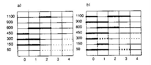
you might have predicted. Some are 'strange'. The two figures below show you
some of the key results. Figure 11 shows you their eyeball estimates of the
conditions which resulted in equilibrium. Over the 120 time intervals their
simulation ran, slow-growing organisms never reached equilibrium on large
islands, but did on small ones when there was no disturbance (indicated by 0 on
the x-axis). They could not reach equilibrium on any islands at higher levels
of disturbance. Fast growing organisms (on the right) could reach equilibrium
on any size island in the absence of disturbance, and with the larger
population size possible on very large islands, could even reach equilibrium in
the face of moderate disturbance levels (i.e. levels 2 and 3).
Figure
10 - indications of relative equilibrium (thick lines) in 10 simulation
runs for islands with different numbers of cells (the y-axis) and different
intensities of disturbance (the x-axis: 0-no disturbance, 1-10% effect, 2-25%
effect, 3-40% effect, 5-75% effect). Part a is for
organisms with 'slow' growth (low clutch size, longer interval between
reproduction, longer lifespan) and part b for 'fast' growing individuals.
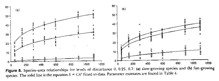
Figure
11 - Species-area relationships for a) slow-growing and b) fast-growing
organisms affected by disturbance. The 3 curves are for no disturbance (top
curves), 25% disturbance effect (middle curves) and 75% disturbance (bottom
curves).
Evident
in Fig. 11 is the community level effect of disturbance. Disturbance lowers the
overall number of species resident, but if there is sufficient time for equilibrium to
have been reached, life history makes a difference. At low levels of
disturbance, the slow-growing species attain a higher diversity. At high levels
of disturbance,
species are not able to remain around long, and a greater diversity can be
achieved by being a good colonizer (a weed, rapid population growth, etc.).
Counter-intuitively, when the actual fitting values for these curves are
assessed, the steepness of the species area curve increases when disturbance is
present, even though overall diversity decreases. What all this tells us is we need
to know more about the effects of disturbance in real communities. The real
world is affected by disturbance on a more-or-less frequent basis, and
conservation models based on an equilibrium paradigm need to be re-considered
to incorporate some indication of the effects of disturbance.
References
Brown, J. and A. Brown. 1977. Turnover rates in insular biogeography: effect
of immigration on extinction. Ecology
58:445
Diamond, J. 1969. Avifaunal equilibria
and species turnover on the Channel Islands of California. Proceeding of the National
Academy of Science 64:57.
Diamond, J. and R.M. May. 1977. Species turnover
rates on islands: dependence on census interval. Science 197:266-270.
Gilbert. 1980. The equilibrium theory of island
biogeography: fact or fiction?. Journal of Biogeography 7:209.
MacArthur, R.H. and E.O. Wilson. 1967. The Theory of Island Biogeography. Monographs in Population Biology, Princeton Univ.
Niering, W.A. 1963. Terrestrial ecology of
Kapingamarangi Atoll, Caroline Islands. Ecological Monographs 33:131-160.
Simberloff, D. 1976. Experimental zoogeography of
islands: effects of island size. Ecology
57:629.
Thornton, I.W.B., R.A. Zan, and S. van Balen. 1993. Colonization of Rakata
(Krakatau Is.) by non-migrant land birds from 1883 to
1992 and implications for the value of island equilibrium theory. Journal of Biogeography 20:441-452.
Villa, F., O. Rossi, and F. Sartore.
1992. Understanding the role of chronic environmental disturbance in the
context of island biogeographic theory. Environmental
Management 16:653-666.
Whitehead, D.R. and
C.E. Jones. 1969. Small islands
and the equilibrium theory of island biogeography. Evolution 23:171.